Indeed, all recent Tevatron searches for the Higgs feature a combination of heavy weaponry: quite advanced statistical methods which include multi-variate likelihoods, neural network classifiers, boosted decision trees, matrix-element discriminants. Hundreds of man-years of work by particle physicists themselves have been spent in the refinement of those tools, as well as in the critical, uncompromising review of the performances that they could show on control samples of data, on simulated event sets, or when tested one against the other.
The situation has evolved a lot in this respect during the last twenty years or so. When I started my career in particle physics neural networks, for instance, were looked at with a lot of suspicion, and despite all evidence that their output could improve search results significantly, the first experimenters who ventured to use them in discovery searches were little short of crucified!
The problem was partly due to the fact that computers were not as powerful as today. Training a neural network could take a month of CPU time, while now in an afternoon you are typically done for a typically sized classification analysis. In a sense, the evolution of technology has naturally caused our statistical methods to evolve synergetically with it. The increased confidence we have acquired in our simulation programs, the so-called "Monte Carlo" generators on which we base our modeling of the detailed characteristics of the signal we search, has been the other important factor in this evolution.
I will leave the story of the developments of advanced analysis methods, as well as of the ensuing controversies (and crucifixions) to another day. What I care to discuss and explain here and in the next part of this piece, providing a couple of examples, is that despite the trends that particle physics has displayed in the recent years, the issue of whether an experiment is seeing a new, unexpected particle in a given dataset remains one where very basic statistics rules. Mind you: little nasty devils hide in the details of basic statistics. We are going to exorcise a couple here.
The basic problem: finding humps in mass distributions
Rest mass is a particle's footprint: its value can be measured by determining the energy and angle of emission of all its decay products. A full reconstruction of the mass is not always feasible; but whenever it is, the signal of a particle decay will universally appear as an enhancement in the number of event counts at a particular value of its reconstructed mass. Such a signal is what physicists improperly call a resonance. What resonated were the constituents of the system before it disintegrated, and not the decay products; but physicists are not philologists, and they use metonymy whenever it simplifies their jargon.
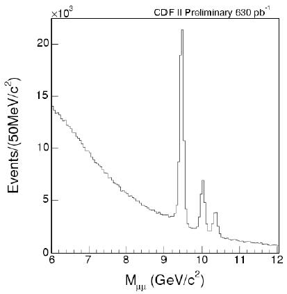
 So, just to clarify what I am talking about here, let me show you a picture that makes my heart miss a beat every time I look at it. The three bumps shown in the graph on the left are three famous resonances, the Upsilon family: these are three of the most common states that a pair of bottom quarks can bind together into.
Those three bumps stand out so overbearingly on top of the smooth, "continuum" background, that no physicist would object to the picture of Upsilon mesons as constituted by a bottom-antibottom quark pair orbiting around one another, and resonating at any of a small set of very characteristic frequencies - the ones corresponding to the Upsilon mass values-, until they find a way to give back to the environment their energy in a decay, producing a pair of muons (in the case of the events displayed) which are then detected and measured.
Seeing a Upsilon meson at a particle collider is commonplace nowadays, but it took the ingenuous minds of Leon Lederman and his collaborators to discover it, thirty-two years ago. Leon was awarded a Nobel prize for that important find, but as far as the experimental analysis technique is concerned, he did not invent anything new: bump hunting had been a favourite field of investigation of particle physicists since the early fifties, when the first hadronic resonances had started to appear in bubble chamber images.
Take the X(3872) meson as a very clear example. That mysterious particle, whose true quark composition is still the subject of debate, was discovered by Belle in 2003 using the decay chain
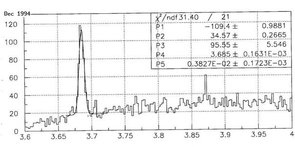
You can make up your own mind on whether my CDF colleagues were too conservative when they neglected to report on that result, by looking at the graph shown below. In it, you can clearly see the Psi(2S) signal (a resonance quite similar to the middle Upsilon bump shown previously, except for being formed by a lighter charm-anticharm quark pair) standing tall on the left, but you may also see a nagging two-bin fluctuation over the smooth background shape, sitting at about 3870 MeV.
Should CDF have called for the observation of a new unknown particle, based on the evidence of that bump alone?

Of course not. The two-bin fluctuation amounted to just a few tens of events, over a background of maybe sixty or seventy: it was simply not significant enough to be meaningful, despite the fact that we now know it was not a fluctuation at all, but a real resonance! To explain why the X at CDF in 1994 was not significant, I am going to discuss below some basic statistical facts which are known by heart by bump hunters.
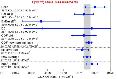
 (Before I do, let me pay justice to CDF, which has taken a very satisfactory revenge with the B-factories on the measurement of the X(3872) particle: As shown in the graph on the right, CDF now holds by far the most precise determination in the world -the fourth bar from below- of the very important mass of the X particle. Why the X mass is so important to determine precisely is explained elsewhere; here just look at the graph on the left, which shows the most recent and precise measurements of the X mass: CDF tops them all! Need I say it is my experiment ?)
Signal significance and the "look elsewhere" effect
Imagine your experiment collects 100 events in a restricted region of a mass spectrum, where on average you expect to see 70 from known sources. Statisticians teach us that event counts follow a Poisson probability distribution function: this means that the intrinsic fluctuation of the observed counts should be measured in units equal to the square root of the counts. For 100 events the statistical error therefore amounts to plus or minus 10 events: this says that if you were to repeat data collection under the same experimental conditions, you would be 63% likely to get a number between 90 and 110.
So if you observe 100 and expected to see 70 events, you are facing a three-standard-deviation excess, more or less like the one shown in the graph above.
Physicists may get excited if a fluctuation in event counts reaches the level of "three-sigma", as they call it. That is dubbed "evidence" for some effect present in the data and not described by our predictions. If, however, the departure of observation from expectation reaches the level of "five-sigma" -five standard deviations away from the expectation-, one talks of "observation" of a new, yet unknown effect. Experience has shown that three-sigma fluctuations do happen in particle physics experiments out of sheer chance (discussing whether they do with the expected 0.3% frequency or at a higher rate might be entertaining, but let us forget the issue now), while "observation-level" excesses are credible indications of a discovery.
Now, consider the mass spectrum shown in the figure above: not only is the clustering of events at 3872 MeV insufficient to reach "observation level": the crucial thing here is that nobody had predicted that a J/Psi plus dipion resonance would sit exactly at that mass value! The problem is well-known to experimental physicists: since, in the absence of a theoretical prediction, the experimenter cannot tell beforehand where an excess might appear in the mass spectrum, the possibility to observe a random fluctuation resembling a signal gets automatically enhanced by the fact that we allow it to appear anywhere. If those 30 excess events are concentrated in a mass region spanning one hundredth of the total width of the explored spectrum, we have to account for that allowance somehow.
A back-of-the-envelope calculation of the mentioned effect is easy to perform: since small probabilities combine additively, the 3-permille probability of the 30-event excess flucutation gets multiplied by the number of places where it might have occurred. A 0.3% effect thus becomes something you should expect to see 30% of the times, and you should retrieve the champagne from the fridge and put it back in the cellar.
(I should probably explain better, to the most curious of you, what I mean when I say that small probabilities "combine additively": the exact way of saying it is that when one searches for the occurrence of at least one of several independent effects, each of them having a very small chance of happening, the total probability is well approximated by the simple sum of each independent probability. Take the example of three simultaneous bets on number zero at three roulette tables: since each has a P=1/37 chance of winning, the above recipe says that your total chance of winning at least one of the three bets is roughly 3P=3/37. The true number is instead computed as one minus the chance to win none of the bets, or
In truth, while physicists usually thrive in order-of-magnitude estimates, when it comes to measures of statistical significance they become really picky. The exact way to estimate the chance that a bump of N signal events occurs is then provided by the study of pseudoexperiments. These are mock mass spectra, each made to contain the same number of entries as the one under test. Entries are extracted at random from a background shape equal to the one observed in the data, ignoring the possibility that a signal is present on top of it.
A search for a Gaussian signal in each of these mock spectra -which, I must stress, do not contain any signal by construction!- then allows to figure out how likely it is that one sees by chance a fake signal of at least N events in the real data: this probability is computed as the number of pseudoexperiments displaying such a signal divided by the total number of pseudoexperiments that have been scanned.
The only drawback of the above technique is that it is heavily computer-intensive: in order to measure very small probabilities one needs to generate very large numbers of pseudoexperiments. However, that is not a big issue nowadays, since computing power has become cheaper than the air we breathe. Pseudoexperiments are now such a standard technique that the most popular statistical package used by particle physicists provides the generation of these mock spectra with a single command.
The "Greedy Bump bias"
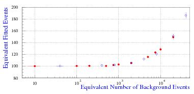
 All the above is so well-known by specialists that I feel a bit ashamed to have reported it here: it is not new, nor original material, and it is not particularly accurate either. However, I needed to provide you with an introduction to the more interesting part of this piece which, unfortunately, has become already longer than it should. Rather than asking you for too much of your precious time in a single chunk, I prefer to defer the discussion of the part which is indeed original (and unpublished) by a few days. Nonetheless, above and below are respectively a unexplained graph and a cryptic but faithful summary of what we will see in the next part: it is an effect which, as far as I know, has not been investigated in the literature (but I would be glad to know otherwise, if you have a reference!). I have dubbed it the "greedy bump bias":
When fitting a small Gaussian signal with a fixed width and a variable mean on top of a large smooth background, the fit usually overestimates the size of the signal. The reason is that the statistical figure of merit of the fit benefits more by fitting a signal larger than the one present in the data, rather than by fitting fewer events. The fit does so by slightly moving the fitted mean away from the true value, finding a positive fluctuation left or right of it. The resulting bias in the number of fitted events appears to be a universal function of the ratio between the number of signal events and the square root of the number of background events sitting underneath it.
So, I hope you will come back for the rest of this post soon!
UPDATE: part II is here.


Comments