

Yet most of the time you only have a hunch of how the PDF looks like: you know it has some general properties, like asymptotes, and location (the mean, which your data sample can provide easily); in most cases you also have an estimate of its variance. But you may be wrong on some details; and they can be paid very dearly, as if you mistake the properties of the PDF your whole inference from the data can be biased, or even completely screwed up.
But what is the PDF exactly? It is a function f(x) of one or more random variables x which you can measure. f(x) may also depend on some unknown parameters, and in that case we write it as f(x;theta), where theta is understood to be a vector of parameters that may change the shape of the function. In many statistical problems (parameter estimation problems, that is), the name of the game is to estimate the theta values from a bunch of data, a sample of x values, written as {x}.
To be a probability density function, our f(x;theta) must have an integral over all the space of the observable x to be equal to 1.0: it must be, in other words, normalized, as it is after all a probability, and Kolmogorov explained back in 1937 that to be a probability you need to have an integral of 1.0 over the observable space.
Further, the PDF is understood to be a function of x, where the theta values are fixed - but you do not know the latter, in most cases! If you know the PDF AND you know the parameters, then you know everything: you can compute the exact probability that you observe some data x.
Perhaps it is useful at this point ot also explain that we have been speaking about the functional form of our PDF f(x;theta) : how it is mathematically written, that is. E.g., a valid PDF is an exponential distribution, f(x;theta) = 1/theta exp(-x/theta). Here theta is the unknown parameter, while x is the data you can measure. The 1/theta factor takes care of normalizing to 1.0 the PDF for all x>0. There exist more functional forms that are valid PDFs than stars in our universe, so let us not try to list more of them here; you got the point.
What I want to get to, in this post that nobody will ever read, is to explain how you could build an approximate model of the PDF for a given problem. Because that is the creative part of a scientist that wants to use a statistical model to learn something of a system. You first build a model of the system, and then proceed to determine its parameters; this may lead you to figure out that the model was not too good, and proceed to improve it. In this iterative process, which is called science, there is a lot of creativity involved - the scientist has to imagine how the details of the problem conspire to produce some mathematical form for the probability density function that describes how frequently they should measure some data from the system.
So let us discuss some random problem here, to describe how the creative process could unfold. The problem I have in mind is based on my experience of today - I had a lecture in Statistics for PhD students scheduled at 10.30 in the morning, but I also had an ECG exam scheduled at 9.30 a few km away. I had warned the students that I might be late, but I had also explained that I would not be able to be precisely estimate how likely it was that I would be annoyingly late, or not show up at all. [It turned out that I was able to make it to my lecture with just 12 minutes of delay.] In reality, I could have given it a try...
We may agree that estimating precisely the time at which I would show up for the lecture is impossible, as this depends on many factors that are out of my control. But then, we do have a way to put together a good model for the probability distribution of my arrival time at the lecture, as I wish to discuss.
First of all: the probability that I make it to the lecture is not perfectly defined - if there is a earthquake so strong that it moves buildings south by 5 meters, does it count if I get at a time T to the place where the lecture room once was, or should I instead consider the time when I do get to the new place where the building sits? And what if the building does not exist any longer?
What I am getting at is that we may need to agree that the probability has an integral that is less than 1, because we subtract from the normalization condition the estimated probability that I do not make it at all there (which can happen for a variety of additional reasons besides the building being leveled - I am dead, or unconscious, or had some other accident that prevents me to physically make it there).
To the admittedly small probability of no-show we may agree to add the probability that the lecture room is so utterly destroyed by some cataclism that I cannot really show up. What is the total? Maybe 0.01 or so? Fine, we can take that as an assumption. So our searched-for f(t) distribution - the distribution of my time of arrival in the lecture room - has an integral of 0.99. We made some progress.
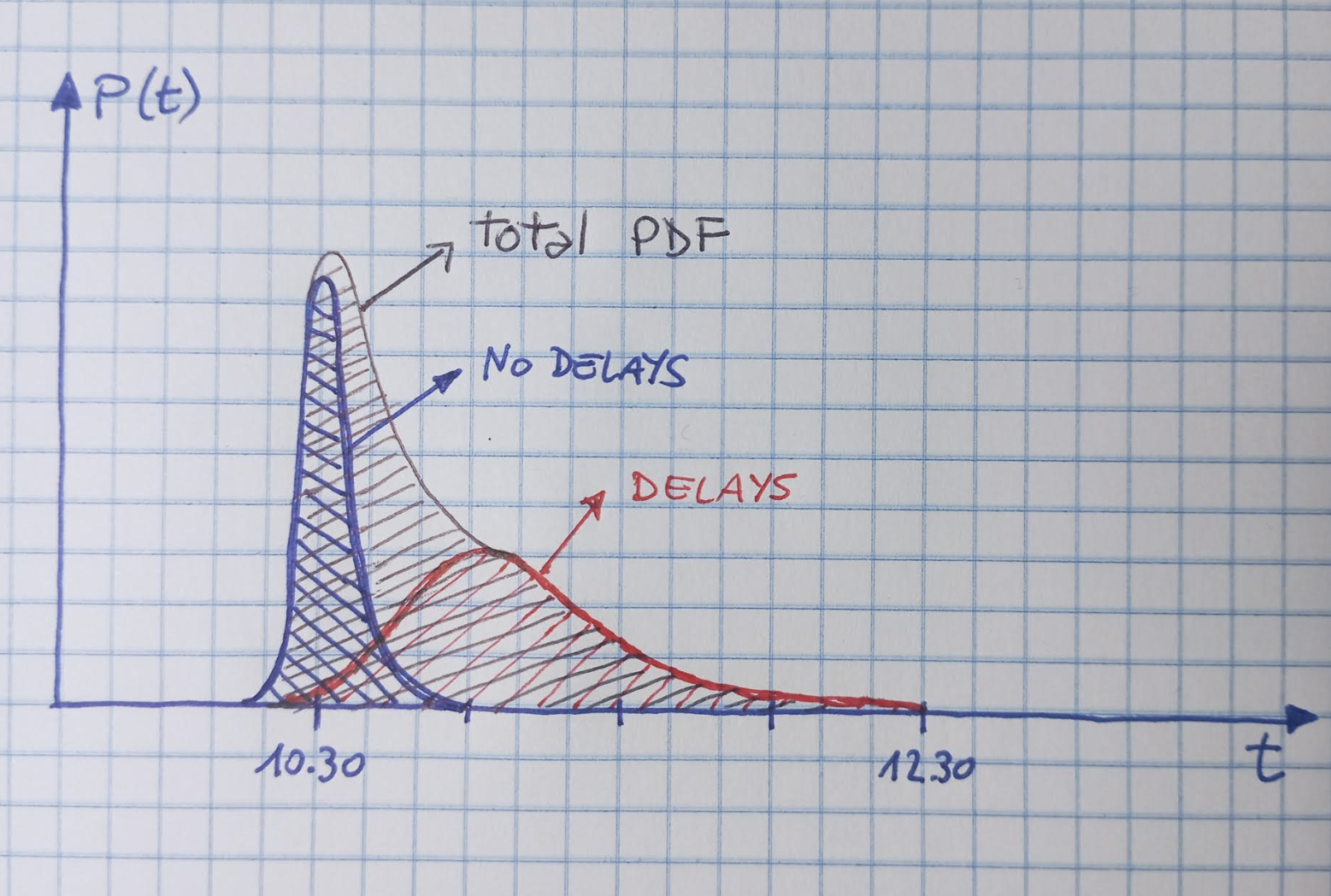
Now, we can consider that if the ECG exam goes as scheduled and I leave the hospital well in time, I will be able to show up at the right time - 10.30AM. Of course my watch could be lagging behind or running a bit fast; or I might meet a colleague just before reaching the room and get there late anyway. We can model the distribution of my arrival time as a gaussian function then, centered at 10.30 and with a sigma of 2 or three minutes, and add to it some tail to the right to signify that there is an increased chance that I am late by a little bit.
But how large is the normalization of this curve? We have to estimate how likely it is that the ECG exam was on time and that I had no other delays such as traffic jams etcetera. Let us say that I believe this can happen 30% of the times, based on previous experience.
What is left is then to model a distribution of time arrivals for the remaining 69% of the cases, when I was indeed delayed. This distribution will have some smooth rise at times later than 10.30AM, and of course also decrease to zero for times so late that there is no point for me to go to the lecture (as all students would have left anyway). Say this time is 12.30, the time of end of my lecture. So this distribution I am trying to model is more or less located in the 10.30-12.30 interval. Its normalization is not 0.69 though: it is smaller, as there is a non insignificant chance that my delay was of more than 2 hours, when I would then decide to not show up at all. Maybe this is a 10% chance, so the normalization of this "delay" distribution should be of 0.59. But what is its shape?
Probably a good hunch at the probability distribution of my time of arrival, in case the medical exam prevented me from being on time, is a gamma distribution - a shape similar to a Gaussian, but with a long tail to the right. This tail will also be dying out quickly (with some smoothing due to my watch not being too precise, as mentioned above) at 12.30 for what we have said before - I just turn on my heels if I figure out I can't be there by the end time. Here is a sketch of how the ingredients might contribute to the expected time of arrival.
As you can see, my evaluation of the relative odds of making it there on time or not do shape the distribution, by giving more or less weight to one of the two humps. But now that we spent all this time trying to construct it, we have to ask: is it important to have tried this exercise? What do we gain by having a functional form for it?
Well, it may not matter so much to my students, although they could have some reason to use the data to decide what to do with their morning schedules [for instance, upon seeing that I predict a 50-percent-ish chance of being late by more than half an hour, they could decide to arrive late themselves, or to just get in the room to check if I am there at 11.00AM and then leave if they do not see me there]. The knowledge of the PDF, however approximate, would allow them to take an informed decision on their action, minimizing what is called a "cost function". But let me omit discussing decision theory here, as the focus is elsewhere.
The real purpose that an exercise of the kind above serves is to show that we can, in most of our daily activities, think in terms of probability; we can "think forward" to all the possible events that may modify the observable future, and build a mathematical model with that. More often than not, the use of the mathematical model - however approximate or even plain wrong that may turn out to be - will be useful for rational thinking and indeed, to take informed decisions. This is, after all, what scientists do!


Comments