The example is meant to have two attractive properties: be analytically solvable in closed form - meaning that one may compute with paper and pencil all the relevant results - and be described by simple-to-interpret graphs. Below I will describe what I came up with, but first let me explain what are the points I wish to focus on.
Over the past 20 years or so, advanced statistical learning techniques have been developed and perfected for a number of applications. Their implementation in physics data analysis has been somewhat slow, but we have eventually caught up, attracted by the large potential gains of those techniques over more standard methods.
The classical setup to which in particular boosted decision trees (BDT) or artificial neural networks (ANN) have been applied is that of a classification task: you have data coming from a background process (the uninteresting part) within which a very interesting signal is potentially hiding. You believe you know the properties of the background and of the putative signal (as e.g. provided by a simulation of the underlying physics and detection procedures), and you wish to exploit those features to devise a selection procedure that be capable of enhancing the signal component in the non-discarded data.
The enhancement can and should be quantified precisely in order to provide a figure of merit to maximize. One then chooses, e.g., the "significance" of the excess of signal events on top of the expected background, conditional to the selection clauses (i.e. on the data passing the selection requirements). I will leave for later an explanation of how a significance estimate can be derived; for now, it suffices to say that it is a function of the expected background and signal events collected by the selection.
The toy model
Now, the point I want to make with my toy example is that nuisance parameters - quantities that affect the correctness of the statistical models describing background and signal - have until recently been by and large ignored when devising procedures aimed at identifying the most performant classification algorithm, as well as choosing their optimal operation point (the value of the classifier output which, by definition, maximizes the expected significance of the signal in data selected to have values larger than that).
The result is that a classifier believed to be the best one in the given application may not be such, and further, that its chosen operating point may not be the one providing the maximum significance, once the effect of nuisance parameters is accounted for (which is an operation done typically after the classification task has ended). The above point is of course what I mean to bring home as a means of introduction to the discussion of classification methods and procedures that do correctly account for nuisance parameters in the optimization task.
Now, let us discuss the model I came up with. Given the excellent properties of the exponential function (in particular its invariance under derivation), I chose a background model described by b(x) = exp(-αx), with α a parameter, and a signal model described by s(x) = exp(x-1). Both b(x) and s(x) are defined in the x interval [0,1], to make things easy and to let them resemble the typical output of a binary classifier.
Of course we need to normalize to unity s() and b() in the chosen support, such that we can correctly identify them as probability density functions (PDF): this will enable useful calculations below. A simple integration of the functions in the [0,1] range provides the normalization factors, as


Hence the PDFs of signal and background are more properly written, in the [0,1] range we chose, as

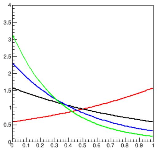
The two functions are shown in the graph below, where s(x) is in red and b(x) is shown in black, blue and green for values of α of 1, 2, and 3 respectively. So far so good, right?

Now, let us imagine that those curves are already the output of a classifier, tasked with separating as well as possible signal from background. Given a value of the parameter α, an ANN (say) will produce a classification score for each event, which will be distributed as shown between 0 and 1; background events are preferentially getting a low score, and will cluster close to zero; on the contrary, signal events will more likely take on larger scores.
Assessing the classification performance: the ROC curve
The way one assesses the performance of a classifier is by constructing what is called a "Receiver Output Characteristic" (ROC) curve. This is a function which connects, for any choice of a selection of data based on the classification score x*, the fraction of signal events accepted by the selection (i.e. those for which x>x*) to the fraction of background events accepted by it. If one considers the classification task in the guise of a hypothesis test for each event, these two quantities may be called "true positive rate", TPR, and "false positive rate", FPR. Of course, the larger x* gets, the smaller get both TPR and FPR; however, the latter diminishes more quickly, so that one gains in terms of the signal fraction of the selected data.
The ROC curve for the three considered b(x) and the single s(x) models shown above can be computed with a simple integration of the quoted PDFs. Sparing you the intermediate (elementary) math, the results are

In order to draw the TPR as a function of FPR in a graph one needs an additional algebraic step, though: both TPR and FPR above are defined as a function of the cut value x*, but we need TPR(FPR) for our graph, such that the TPR is the vertical value (ordinate) to which an abscissa valued FPR corresponds. This can be achieved by some additional simple algebra, which I will spare you (hint: define FPR=t, work out an expression for e^(x*) as a function of t, and then substitute in TPR).
The result is shown in the graph below. As you can see, the three curves all rise from 0 (at FPR=0) to 1 (at FPR=1). Please note, the abscissa is not x*, but a function of it. In fact, for FPR=1, TPR=1 we are at x*=0 - no selection being made, all background is classified as good, as is all signal; and for FPR=0, TPR=0 we are at x*=1 - all events are discarded.

.
Now, the three curves above can be thought of as different performance functions for a classifier that knew the background to be distributed as the blue model in the previous graph (i.e. for α=2) when in fact the background data come in distributed by a different value of the parameter: for α=1 the performance is lower (black curve), while for α=3 it is higher than expected (green curve). Now, if you think of α as a nuisance parameter, you see that if you where to take a decision on the working point x* of your selection based on e.g. the TPR you want your selection to have (say, 0.5, a 50% efficiency on signal events), you would incur in a FPR which is different from what you believe it is given your trust on the background model (i.e. your belief of α=2).
Numerically, the value of FPR corresponding to 0.5 in TPR for the blue curve is of 0.178083, and is achieved by cutting at x>x*=0.620115; but that selection, if the true value of α was in fact 3, would correspond instead to a FPR=0.111377; and for α=1 it would correspond to FPR=0.268941.
More to the point, a modeling uncertainty (a nuisance parameter affecting the PDF of your background) would induce you to take an incorrect decision on which architecture of your classifier would be the most beneficial, as your ROC curves would be unreliable.
A further clarification of the fact that what we call "optimization" of the working point of a classifier is not such, in presence of nuisance parameters, can be obtained by investigating how the significance of the signal we isolated by selecting data with classification score above x* varies if we do not control the background model well enough. For this, we need to define the significance more quantitatively than I did above.
In a situation common to high-energy physics and astrophysics, we collect data from background an signal by exposing our detector to a given data-taking period. Both background and signal come in at random, at a fixed rate. These are therefore Poisson-distributed event counts. If we isolate, by a selection based on e.g. a classification score, a subset of the data (N events) where we expect only a certain amount of background B, but in reality a signal S is also present, we will in general observe an excess of events, N>B. A significance measure of the observed excess, N-B, can be obtained by a procedure which is made up of two steps.
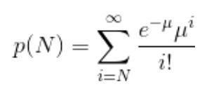
In the first step, we evaluate how probable is to observe at least as many events as N if they came from the background source alone. This is computed as the tail probability of a Poisson distribution of mean B, i.e. the integral of P(N) from N to infinity:

Once we have that p-value, we can convert it to a Z-value by inverting the formula below, which equates p(N) to the tail integral of a unit Normal distribution:

The Z-value is thus a mathematical map of the p-value: it basically allows us to easily speak of very small p-values (say, p=0.000000293) as small numbers (the corresponding Z=5) without having to deal with large number of decimal zeroes, not differently from the ease which is provided by the suffixes giga-, tera- or nano-, pico- that are used for e.g. measures of data size (gigabytes) or distances (nanometers). It is a very convenient quantity to use for optimization of our Poisson counting experiment, in fact.
Now, if we want to compute the tail probability resulting from observing N events when B are expected, as a function of the selection cut x* in our toy setup, we need first of all to specify the all-sample background and signal rates, i.e. the number of events expected before we select the data.
Let us assume the background produces on average, in the collected data, B=400 events, and that the signal produces S=20 events. If we do not use the classifier, we are looking at an observed 420 events with an expectation of 400: a small excess, not significant -in fact, it corresponds roughly to a Z value of 1, as the R.M.S of a Poisson of mean 400 is equal to sqrt(400)=20.
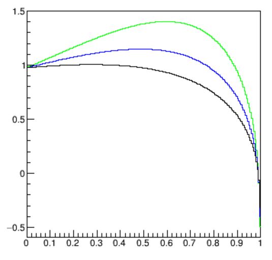
A not-so-straightforward calculation involving Gamma functions is needed to extract the p-value from the integrals of the selected data based on our b(x) and s(x) models. The computer helps draw the resulting significance curves, shown below for the three choices of α and B=400 events, S=20 events in total.

As you can see, the more "peaky" is the background PDF at zero (corresponding to higher values of α), and the higher the significance may get if you select data at non-zero values of x*. But here you also notice that the optimal cut value is different depending on the value of the nuisance parameter: the optimal selection strongly depends on the detail of the background model. The graph shows that optimality is reached at x*=0.60 , 0.49, or 0.28 if α is equal to 3,2, or 1. This of course means that an imprecision of your background model will cause your whole optimization procedure to be deeply flawed!
Further, let us compare the above curves with ones obtained from a different signal rate, S'=5. Until now we have assumed we knew the rate of the signal we were looking after, but it is, after all, another potential nuisance parameter implicitly affecting our model. We may investigate what happens if we got it wrong, too. In the figure below you can see what happens if we optimized our search assuming S=20 while in fact S'=5: of course all Z-values decrease by a large amount, but of relevance is also the fact that they reach their maxima at different values of the cut variable x*, precisely at 0.56, 0.44, and 0.22 for the three values of α.

In summary, any optimization worthy of its name, in a classification task, should include the consideration of all possible sources of uncertainty affecting the inputs to the problem. Nuisance parameters may modify the PDF of the classes or the relative or absolute rates of the events in the data with respect to what is assumed by our models, and they directly affect the relative merits of our decisions, if we do not account for them.
Looking further: incorporating nuisance parameters in the learning process
But how can we account for them when we use complex machine learning tools, such as e.g. multi-layer neural networks? The issue has been studied for a long time in the context of what is called, in computer science, as "domain adaptation": for example, you have a neural network that is trained to distinguish spam from genuine e-mails based on the words contained in the messages. Now you feed the NN with text from product advertisements, and try to see if it can correctly flag ones that are deceptive or fraudolent. If the NN is capable of doing so, it is said to possess a measure of domain-aspecificity: it is robust to variations of the domain to which it is applied.
In fundamental physics the problem is more circumscribed and better analytically described than in the general setting mentioned above. Nowadays there is a dozen of different techniques that has been tried with some success to problems of relevance to our research field, and a few are definitely promising. These techniques are based on e.g. extending the feature space to include the nuisance parameters in the training - an useful but sometimes impractical solution; or on the adversarial setup of different NNs, one of which tries to maximize the classification performance and a second one that tries to second-guess the value of the nuisance parameters.
A recent idea on which I published a paper last year with my bright student Pablo de Castro is instead based on directly incorporating in the loss of the classifier a notion of the final objective of the classification task, a sort of "awareness" of what the classification score is going to be used for. Using the inverse of the Fisher information for this produces fully optimal results. This is I believe the most promising avenue on the way to achieve a full end-to-end optimization of our classification solutions.


Comments